Borehole Strainmeter Overview
Background
Borehole strainmeters (BSM) are extremely sensitive to change in the earth around them, capturing a rate of deformation that bridges a measurement gap between seismometers and high precision GPS (e.g., GPS; Figure 1 - frequency of deformation). This makes BSMs ideal for measuring deformation spanning seconds to weeks. Examples of signals the instruments excel in measuring include earth tides, volcano deformation, postseismic earthquake deformation, and slow fault slip events. A few cool papers that explore such phenomena can be found here.

FIgure 1. Created by John Langbein, USGS, showing the rate sensitivity of seismometers, strainmeters, high rate GPS, and SAR.
The global distribution of stations supported by Earthscope is plotted up in Figure 2 for reference. All are located near active plate boundaries or volcanic regions, and most were established as part of the Plate Boundary Observatory (PBO) project from 2005 to 2008 (Hodgkinson et al., 2013). Other collaborative project regions include the Geophysical Observatory at the North Anatolian Fault (GONAF) in Turkey and the Alto Tiberina Near Fault Observatory (TABOO-NFO) in Italy. The go-to spot for BSM information, documentation, etc. is this page and associated sub-pages.

Figure 2. Map of BSMs supported by Earthscope.
Strain Review:
The strainmeters measure a change in length. As such, they measure the spatial derivative of displacement. In contrast, seismometers measure the time derivative of displacement and GPS measure displacement. Strain itself is dimensionless, for example:
10-6 = 1 microstrain (ms) = 1 ppm = 1 mm lengthening of a 1 km baseline
10-9 = 1 nanostrain (ns) = 1 ppb = 1 mm lengthening of a 1000 km baseline
The sign convention for us will be:
Increased length → extension = positive strain
Decreased length → contraction = negative strain
Likewise,
Increased area → expansion = positive strain
Assuming small strains, we can apply “infinitesimal strain theory” in a state of plain strain, with assumed deformation only in the East(x)/North(y) plane. Therefore, only strain components \(e_{xx}\), \(e_{yy}\), and \(e_{xy}\) are considered, with \(e_{zz}=e_{zx}=e_{zy}=0\). The normal strains, \(e_{xx}\) and \(e_{yy}\), act perpendicular to the plane, and the shear strains act along it.

Cube showing the directions of strain, with strain in the z direction = 0.
In terms of displacement (u), the strain is expressed as: \( e_{ij}= \large \frac{1}{2} \left[\frac{\partial u_i}{\partial x_j}+\frac{\partial u_j}{\partial x_i}\right]\) \(i,j = x,y = E,N\)
For plain strain in the x/y plane, \(e_{xx}\) and \(e_{yy}\) represent contraction or extension, and \(e_{xy}\) shear strain (as pictured in the image below) measures change in the angle of the body. The engineering shear strain (commonly \(\gamma_2\) or \(2e_{xy}\)) is defined as (\(\alpha + \beta\)), or, the change in angle of \(\overline{AC}\) and \(\overline{AB}\); equivalently, \((\alpha + \beta)=\frac{du_x}{dy}+\frac{du_y}{dx}=2e_{xy}\).
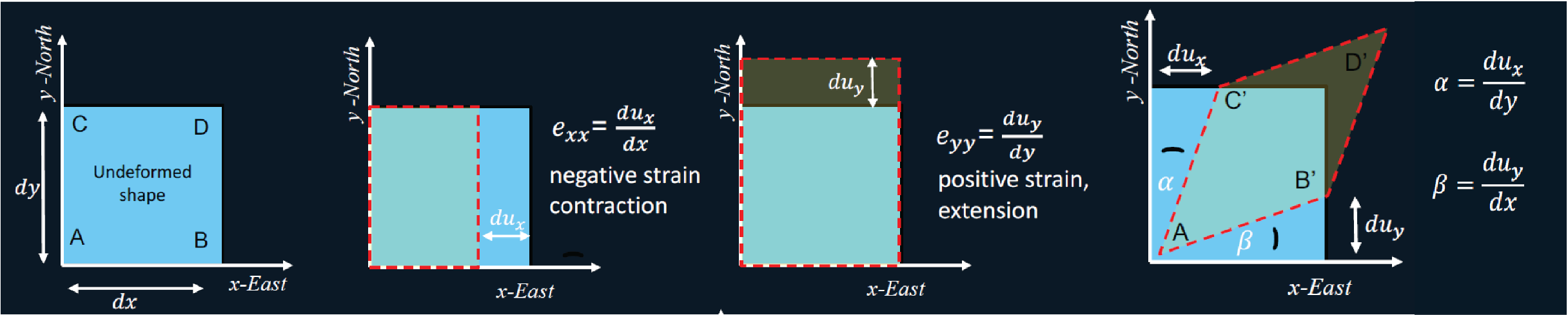
Plane strain.
Instrumentation
The Gladwin Tensor Strainmeter (GTSM; Gladwin, 1984) is the common type of borehole strainmeter managed by Earthscope, so we focus much of this package on that specific design. The instrument, precise to nanostrain levels (the equivalent of shortening a 1 km long baseline by 1 mm!), is typically installed at a depth of ~100 m in a ~10 cm diameter borehole to minimize surface noise. The 2 m-long instrument consists of 4 stacked gauges that measure horizontal linear strain at different angles (Figure 3). The actual unit of measure is a change in capacitance between a fixed plate and a mobile plate that moves with the borehole wall, which is converted to a linear change in distance (Figure 4). Typically, BSMs are collocated with several instruments, including possible pore pressure sensors, thermometers, barometers, rain gauges, tiltmeters, seismometers, and GPS/GNSS stations.
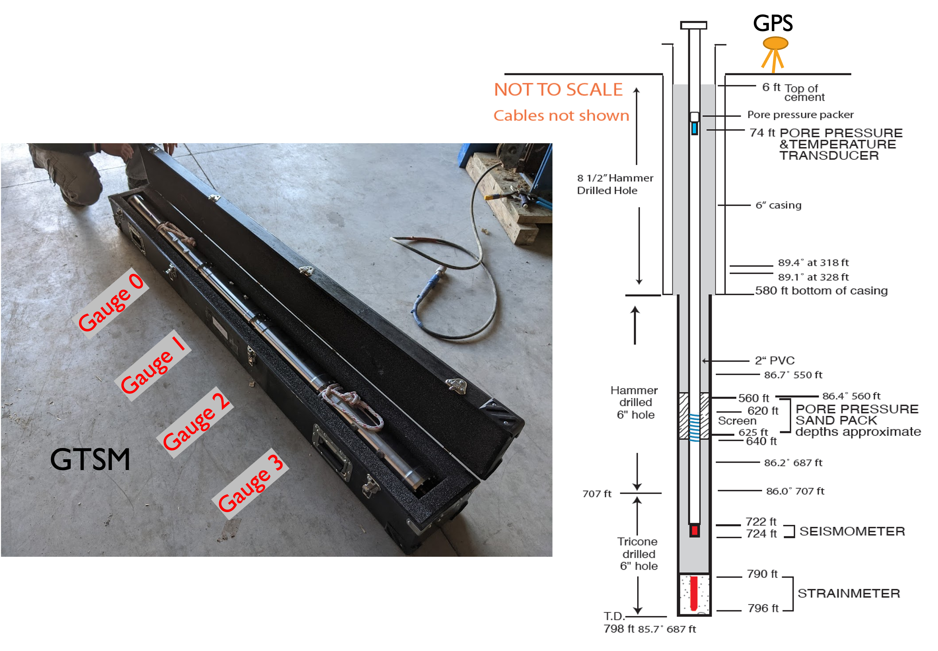
Figure 3. GTSM-type BSM and an example of a station schematic, with multiple instrument types.
Linearization and Calibration
Prior to use in geophysical applications, the raw BSM gauge data must be converted to a unit of linear strain, scaled, and oriented to resolve the full horizontal strain tensor in the east-north reference system. Unit conversion is achieved through linearization, a simple calculation from the 4 raw gauge strains in counts to microstrain (Figure 4).

Figure 4. BSM cross-section depicting the orientation of each gauge, with a drawing of a single gauge. The linearization equation printed below the figure converts raw gauge strain to counts.
On a single gauge, positive change is associated with extension. Calibration scales and orients the four gauge strains to regional areal (east+north strain), differential shear (east-north strain), and engineering shear (east/north strain) strains. Because of their proximity to the surface, vertical strains are assumed to be zero. In practice, some contamination from vertical strain may occur that requires additional consideration in analyses (see Roeloff’s, 2010; Hanagan et al., In Prep for more detail). Figure 5 depicts the regional strain conventions associated with positive change.
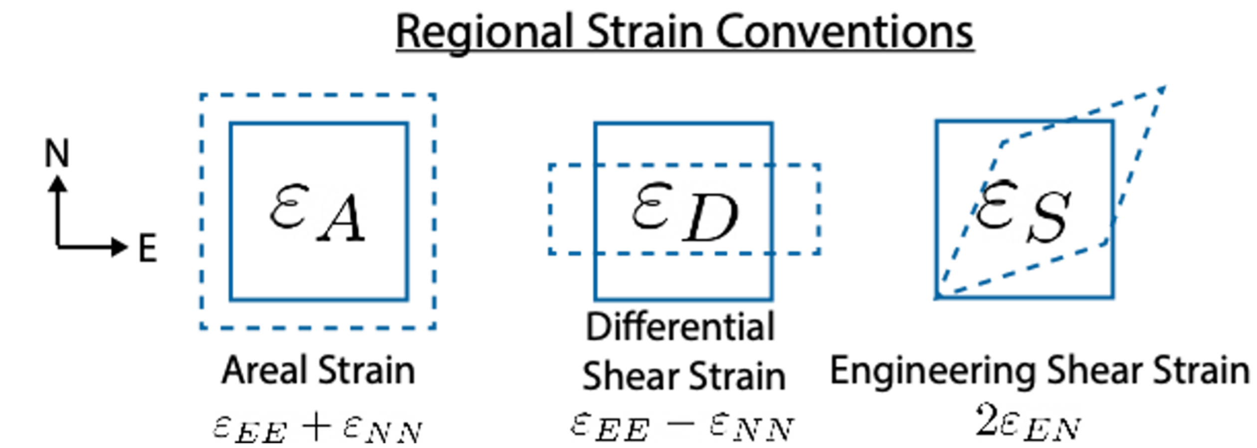
Figure 5. Regional strain conventions in the East/North reference system for plane strain. The solid lined polygons represent the undeformed state, and the dashed polygons represent the deformed state associated with positive changes in strain.
Calibration is achieved through application of an orientation matrix (A) to the gauge strains (EGauge):
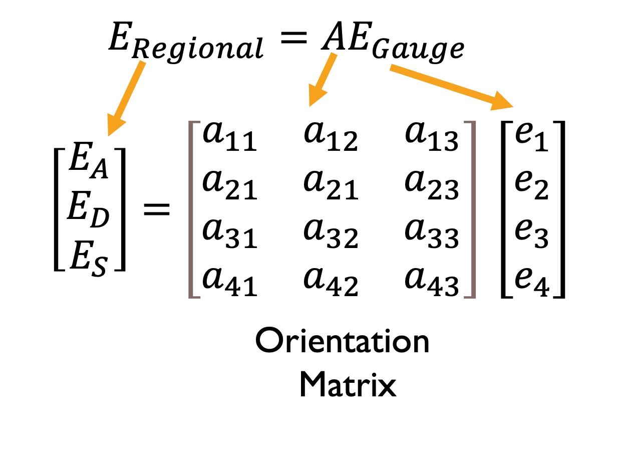
The matrix can be calculated through various methods, two of which are the most common: (1) the manufacturer’s or lab Calibration, and (2) tidal calibration. The lab calibration contains information on the gauge orientation at install, and coupling coefficients derrived from several assumptions (e.g. Hodgkinson et al., 2013). Often, the lab calibration assumptions fail, so alternative calibration is desired. BSMs are ideal at measuring deformation related to tidal forcings. The solid earth tides are well-known, so, often the instruments are calibrated by comparing the predicted and observed earth tides, provided that the instruments are far inland from the coast where ocean loads do not comlicate the predicted tidal strain. More information can be found in the calibration notebooks (need to make these available, with refs to lit).
Common Signals for Correction
[To-do: Change to Data Processing Overview with data processing workflow schematic]
Common signals that can mask, alter, or pose as other signals of interest (e.g. slow slip events) include the long term borehole curing trend, tidal response, barometric pressure fluctuations, rainfall, and sporadic offsets that sometimes occur on a single gauge without know cause. Corrections for the first three (trend, tides, and barometric pressure) are routinely provided in the standard processing workflow. The trend should be evaluated for the timeframe of interest, and, often, a linear trend is sufficient to correct the data after initial grout curing following install has subsided.The tidal amplitudes and phases are determined for each gauge for several constituents (O1, M2, P1, K1, N2, and S2), and are forward modeled and provided to correct the time series. The barometric pressure correction is assumed linear, and predetermined coefficients are multiplied by the colocated surface pressure sensor data for the pressure correction. When available, this can be completed for pressure correction at a rate of 30 minutes, with interpolation to the strain data period, though for several stations 1 sps pressure sensor data is available. Rainfall response on each instrument and even individual gauges of the same instrument can vary due to comlex local hodrogeologic conditions; while no corrections are provided for rainfall, a surface sensor collects 30-min data on cumulative rainfall for comparison. Finally, offset corrections may be provided for jumps in the timeseries regardless of their origin. The user should assess which offsets they deem necessary to correct for. More information is available for utilizing the coding tools and data in the subsequent pages and example notebook files.
References
Gladwin, M. T. (1984). High‐precision multicomponent borehole deformation monitoring. Review of Scientific Instruments, 55(12), 2011-2016. https://doi.org/10.1063/1.1137704
Hodgkinson, K., Langbein, J., Henderson, B., Mencin, D., & Borsa, A. (2013). Tidal calibration of plate boundary observatory borehole strainmeters. Journal of Geophysical Research: Solid Earth, 118(1), 447-458. https://doi.org/10.1029/2012JB009651